
AI Agent Deployment and Scaling: A Production Guide
Deploying an AI agent from a prototype to production introduces challenges that rarely surface during development. The difference between a working demo and a reliable production service comes down to infrastructure design, concurrency handling, failure recovery, and observability — not model quality alone.
This guide covers the practical decisions teams face when moving AI agents into production at scale.
Why Production Deployment Is Harder Than You Expect
Local prototypes run a single agent against one input at a time. Production requires handling thousands of concurrent sessions, recovering from transient API failures, managing token costs under variable load, and maintaining response quality as traffic patterns change.
| Mistake | What Happens | Why It Is Easy to Miss |
|---|---|---|
| Underestimating concurrency limits | API rate limits hit, requests queue unpredictably, latency spikes during traffic bursts | Development traffic is low and consistent; production bursts are uneven |
| Assuming single-model architectures scale linearly | Cost explodes as session count grows; some tasks need different models but the pipeline routes everything to the primary | Single-model cost projections look correct until traffic exceeds the original sample |
| Ignoring state serialization across failures | Agents lose context after a restart, forcing users to repeat entire flows | Prototypes rarely experience mid-session failures |
| Running all agents on identical infrastructure | High-cost reasoning models compete with lightweight agents, degrading both categories | Resource sharing looks efficient until latency SLOs are defined |
Infrastructure Patterns for AI Agent Deployment
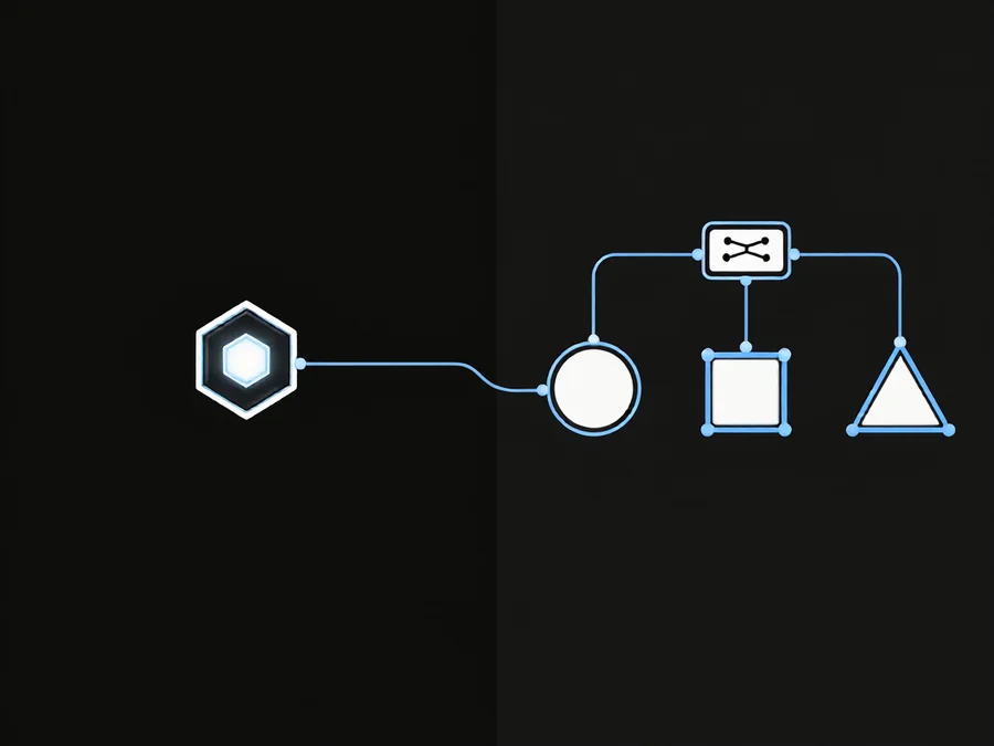
Production AI agent deployments typically follow one of three architectural patterns.
Pattern 1: Serverless Function per Session
Each session runs inside a stateless function invocation. State is externalized to a database or vector store. This pattern scales instantly to meet traffic spikes but incurs cold-start latency of 200–800ms per invocation.
Best for: Variable traffic with burst patterns, event-driven workflows, low-to-medium concurrency workloads.
Pattern 2: Long-Running Service with Connection Pooling
A persistent service maintains long-lived connections to LLM providers. Sessions are managed as in-process objects. This minimizes latency but requires careful connection lifecycle and memory management.
Best for: Steady-state high-concurrency workloads, low-latency requirements, tight turn-around expectations.
Pattern 3: Hybrid Queue-Based Architecture
Incoming requests are enqueued and processed by worker processes. Each worker maintains its own session state while the queue provides backpressure and retry semantics. This decouples ingestion from processing and makes failure recovery deterministic.
Best for: High-throughput pipelines, async workflows, systems that must guarantee eventual completion.
Concurrent Request Handling and Rate Limit Management
LLM providers enforce rate limits expressed in tokens per minute (TPM) or requests per minute (RPM). A production deployment must respect these limits without sacrificing user experience.
Token-Aware Request Budgeting
Before queuing a request, estimate the token budget it will consume. Short-input tasks cost far less than long-context reasoning tasks. Budget allocation should reflect this variance rather than treating every request as equal.
Exponential Backoff with Jitter
When rate limits are approached, use exponential backoff with random jitter to avoid the thundering herd problem — where all retrying clients resume simultaneously and trigger the limit again.
Multi-Provider Failover
Route high-priority traffic through a primary provider and fall back to a secondary when limits are reached. This requires a unified abstraction layer that normalizes API responses across providers.
Practical tip: Monitor your effective RPM utilization as a percentage of your limit. A utilization plateau above 80% for more than five minutes signals that you need either a limit increase or a routing adjustment.
Error Recovery and Resilience Patterns
Production AI agent systems fail. The question is how gracefully they recover.
Checkpoint-Based Session Recovery
Every significant state transition should be persisted as a checkpoint. If a session is interrupted, the system resumes from the last committed checkpoint rather than restarting from scratch. Balance checkpoint granularity: too coarse means maximum rework on failure; too fine means excessive write overhead. A balanced approach checkpoints after each tool-use completion and after every three to five LLM interactions.
Graceful Degradation Under Provider Outage
When a primary provider is degraded, continue serving users with reduced capability — falling back to a slower model, serving cached responses for repeat queries, or deferring non-critical tasks to a retry queue.
Circuit Breakers for Cascading Failure Prevention
A circuit breaker tracks failure rates per provider. When failures exceed a threshold within a sliding window, the breaker opens and short-circuits further requests. This prevents a degraded provider from consuming all available resources.
| Pattern | Trigger | Action | Recovery |
|---|---|---|---|
| Checkpoint resume | Session interruption or worker crash | Restart from last persisted state | Automatic on worker recovery |
| Provider fallback | Primary provider error rate > 5% | Route to secondary provider | Automatic when primary recovers |
| Circuit breaker open | Failure rate > 20% in 60s | Reject requests to failed dependency | Half-open probe after cooldown |
Scaling Strategies: Horizontal vs. Vertical
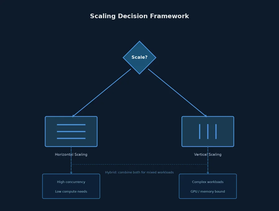
Scaling involves two dimensions: handling more concurrent users and handling more complex individual requests.
Horizontal Scaling: Adding Worker Instances
Horizontal scaling distributes sessions across multiple workers. This is the most straightforward path for stateless or externally-stored-state architectures. The ceiling is determined by downstream dependencies — LLM API rate limits, database connection pools, and vector store throughput.
Vertical Scaling: Increasing Per-Worker Capacity
Vertical scaling increases capacity through larger memory, faster CPUs, or GPU acceleration. Relevant when workflows are compute-intensive — large document processing, complex reasoning chains, or multiple simultaneous LLM calls per session. Vertical scaling has diminishing returns once the bottleneck shifts to an external API.
Hybrid Scaling Decision Framework
- If LLM API rate limits are the bottleneck: horizontal scaling alone will not help; you need multi-provider routing or a higher tier.
- If local compute is the bottleneck: horizontal scaling distributes load effectively.
- If database or vector store throughput is the bottleneck: vertical scaling or read-replica separation is more effective than adding workers.
- If queue depth is growing under load: you likely have both compute and downstream bottlenecks.
Rule of thumb: Measure the utilization of each layer before scaling. If only one layer is near saturation, scale that layer first.
Monitoring and Observability
Three metric categories are essential for production agent observability.
Model Performance Metrics
Track latency percentiles (p50, p95, p99) per model, token consumption rates per session, and error rates by category. Distributional shifts in p99 latency are more actionable than mean latency changes.
Business Outcome Metrics
Task completion rate — the percentage of sessions reaching successful conclusion — is the primary metric. Secondary metrics include escalation rate to human operators and average sessions per task.
Cost-per-Outcome Metrics
Total spend is a lagging indicator. Cost per completed task, cost per session, and cost per inference call provide actionable signals for optimization. Track these per workflow type and per model.
Common Pitfalls in Agent Scaling
Pitfall 1: Assuming linear cost growth. Token consumption does not scale linearly with concurrency because longer conversations accumulate context that grows with each turn.
Pitfall 2: Over-optimizing for average latency. User satisfaction is determined by worst cases, not the mean. A system that responds in 2 seconds for 95% of requests but 30 seconds for the remaining 5% will feel slow to everyone.
Pitfall 3: Ignoring state synchronization costs. Race conditions, lock contention, and write amplification become dominant factors as concurrency increases.
Pitfall 4: Deploying without synthetic load testing. Real traffic reveals problems that unit tests cannot. Run load tests simulating realistic traffic patterns before exposing the system to production traffic.
Implementation Checklist
- Infrastructure pattern selected with documented rationale.
- Concurrency budget defined — max concurrent sessions per worker and per-provider rate limit allocation.
- Error recovery paths tested — simulated provider failures and worker crashes verified.
- Multi-provider routing configured and failover tested.
- Monitoring dashboards deployed — latency, token consumption, error rates, and business outcomes visible in real time.
- Synthetic load test completed — bottleneck layers identified and scaling decisions documented.
- Cost-per-outcome baseline established for optimization tracking.
- Circuit breakers and backpressure rules configured for cascading failure protection.
Frequently Asked Questions
How many concurrent agent sessions can a single worker handle?
Typically 50–200 for short-turn conversations on I/O-bound workers, or 10–30 for compute-intensive workflows with long context windows. Measure your actual bottleneck before setting targets.
Should I use the same model for all agent tasks?
No. Routing different task types to appropriately sized models reduces cost and improves latency. Use smaller models for classification and formatting; reserve larger reasoning models for complex multi-step workflows. A well-designed router can direct 60–80% of requests to cheaper models.
How do I handle sudden traffic spikes without over-provisioning?
Combine queue-based request buffering with horizontal autoscaling. Set the autoscaler target to maintain a buffer — scale up when queue depth exceeds 2× the expected average, not when it reaches zero. This prevents thrashing between scale-up and scale-down events.
What is the minimum viable monitoring setup?
Track request latency percentiles, token consumption per hour, error rate by category, and task completion rate. These four metrics answer: Is it fast enough? Is it affordable? Is it failing? Is it succeeding?
When should I choose a queue-based architecture?
Choose queue-based when workflows are asynchronous, when you need guaranteed completion regardless of traffic, or when you want sophisticated retry and prioritization logic. Choose direct-request when latency is critical and volume is predictable. Many systems start direct and migrate to queues as complexity increases.
Conclusion
Deploying AI agents into production is fundamentally an infrastructure engineering problem. The patterns that distinguish stable deployments — checkpoint-based recovery, multi-provider routing, hybrid scaling, and outcome-focused monitoring — address the realities of distributed systems, not model capabilities.
Start with the implementation checklist, measure your actual bottlenecks before scaling, and treat cost-per-outcome as your primary optimization target. For teams looking to build production-grade AI agent systems with reliable deployment patterns, SmaugBrain provides the infrastructure and orchestration layer that handles many of these concerns automatically.